This project focuses on using Neural Radiance Fields (NeRFs) to reconstruct 3D structures programmatically from 2D images taken from various perspectives. By leveraging deep learning and computer vision techniques, NeRFs enable high-quality, photorealistic 3D renderings with detailed lighting and geometry.
We will start with generating 2D NeRFs, which is a simplified version of NeRFS to get us started. The goal is to feed one image to train a network and the network should be able to return the color when prompted by a specific pixel in the image.
The core of our implementation is a Multilayer Perceptron (MLP) designed to take 2D pixel coordinates as input and output RGB color values. To achieve this, the model utilizes Sinusoidal Positional Encoding (PE), which expands the 2D coordinates into a higher-dimensional representation. This encoding enhances the model’s ability to learn complex spatial patterns by including higher-frequency information.
The MLP consists of multiple fully connected layers with non-linear activations (ReLU), followed by a final Sigmoid activation layer to ensure that the output RGB values remain in the range [0, 1]. Normalization of input image data is critical—pixel values are scaled from [0, 255] to [0, 1], aligning with the output constraints. For hyperparameters, we chose to use an Adam optimizer with lr = 1e-2, batch_size = 10000, and num_iterations = 2000.
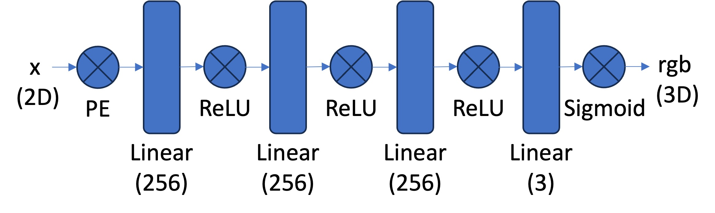
Model Architecture
Model Architecture:
This architecture allows the MLP to represent complex spatial patterns and predict the color of any pixel in the image.
To optimize training on high-resolution images, we implemented a custom dataloader that randomly samples a subset of pixels at each iteration. This approach allows us to be sample efficient and allows the model to learn what the image looks like without seeing every possible pixel. This approach becomes more important when we do 3D NeRFs where feeding the model every posible point is intractible.
How It Works:
N random pixels from the image.Loss Function:
We used Mean Squared Error (MSE) as the loss function to quantify the difference between the predicted RGB values and the ground truth. MSE is simple and effective for measuring pixel-wise reconstruction quality.
Optimizer:
The model was trained using the Adam optimizer with a learning rate of 1 × 10⁻². Adam's
adaptive learning rate ensures efficient convergence even with non-linear activations and positional encodings.
Metric:
While MSE measures reconstruction accuracy during training, Peak Signal-to-Noise Ratio (PSNR) is used as the primary evaluation metric. PSNR is better suited for comparing image quality and is calculated from the MSE using the formula:
PSNR = 20 × log10(1 / sqrt(MSE))
PSNR values provide a clearer picture of the network’s ability to reconstruct fine details as training progresses.
We then trained the model using our dataloader and we can see the predicted image being progressively better as we increase step size.
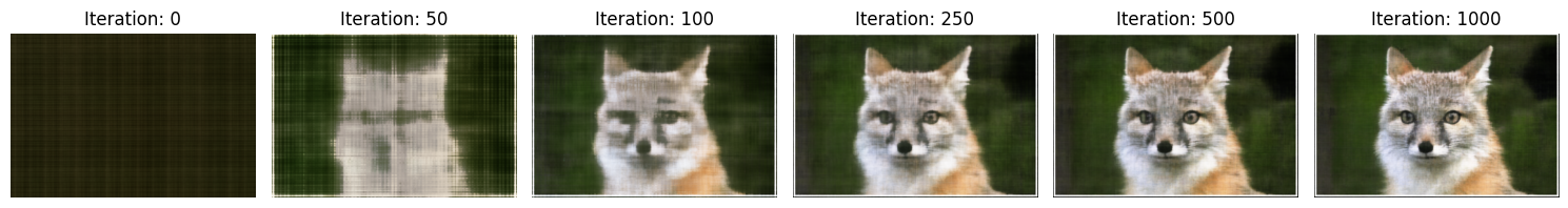
We can see this improvement in quality reflected in the PSNR as well through a quantitative graph:
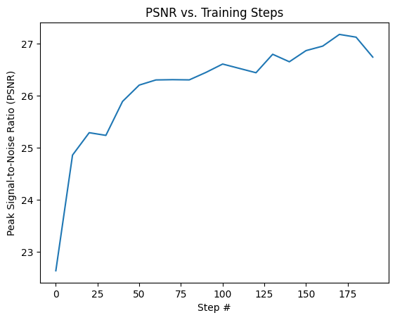
PSNR for Fox Image
We tried running it on a different image as well using the same architecture and hyperparameters as well. This method should work well for other images, too.
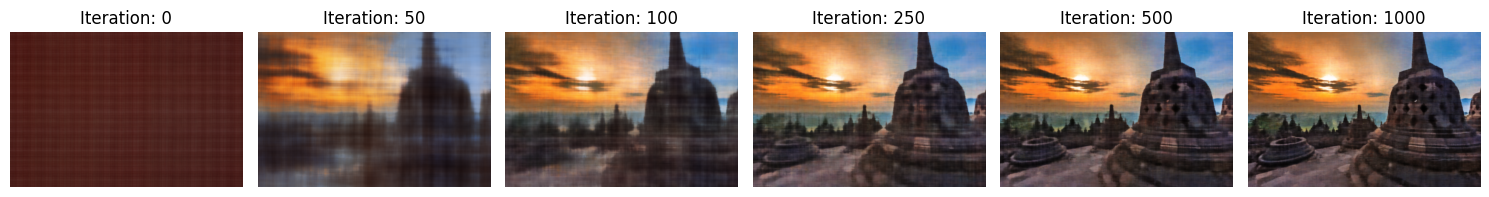
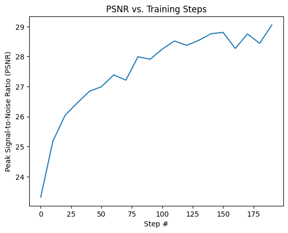
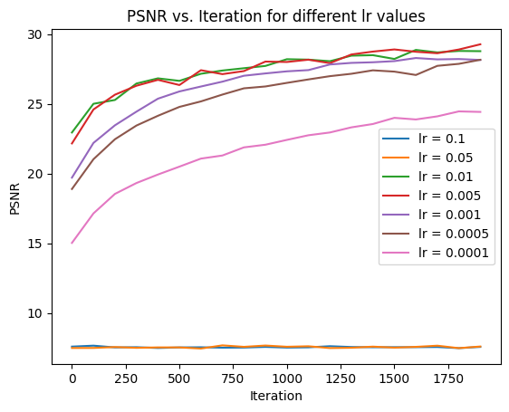
PSNR for Temple Image
Exploring Hyperparameters:
We experimented with two key hyperparameters:
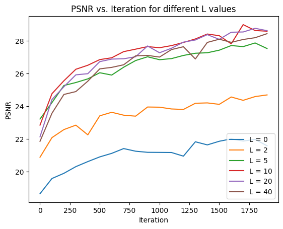
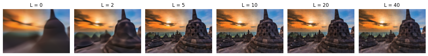
Varying L
After trying varying values of L = [0, 2, 5, 10, 20, 40], we saw that increasing L generally improves the network’s ability to capture finer details but increases model complexity which may lead to slow model training and potential overfitting if set too high.
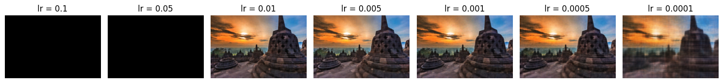
Varying LR
After trying varying values of lr = [1e-1, 5e-2, 1e-2, 5e-3, 1e-3, 5e-4, 1e-4], we saw that an lr value between 0.01 and 0.001 yielded the best results. This could be because the model never gets to a minima if the lr is set too high and it reaches the minima too slowly when lr is set too low.
We can now continue to making fully 3D NeRFs, which take in 2D images from different perspectives and generates a 3D structure out of them. The approach is similar to the 2D NeRFs where we query the model for the color at a particular point, but now we query with a 3D point alongside a ray direction and receive both the color and density of the point.
To convert camera coordinates to world coordinates, we use the camera's extrinsic matrix, which encapsulates the rotation and translation needed to align the camera's coordinate system with the world coordinate system. Specifically:
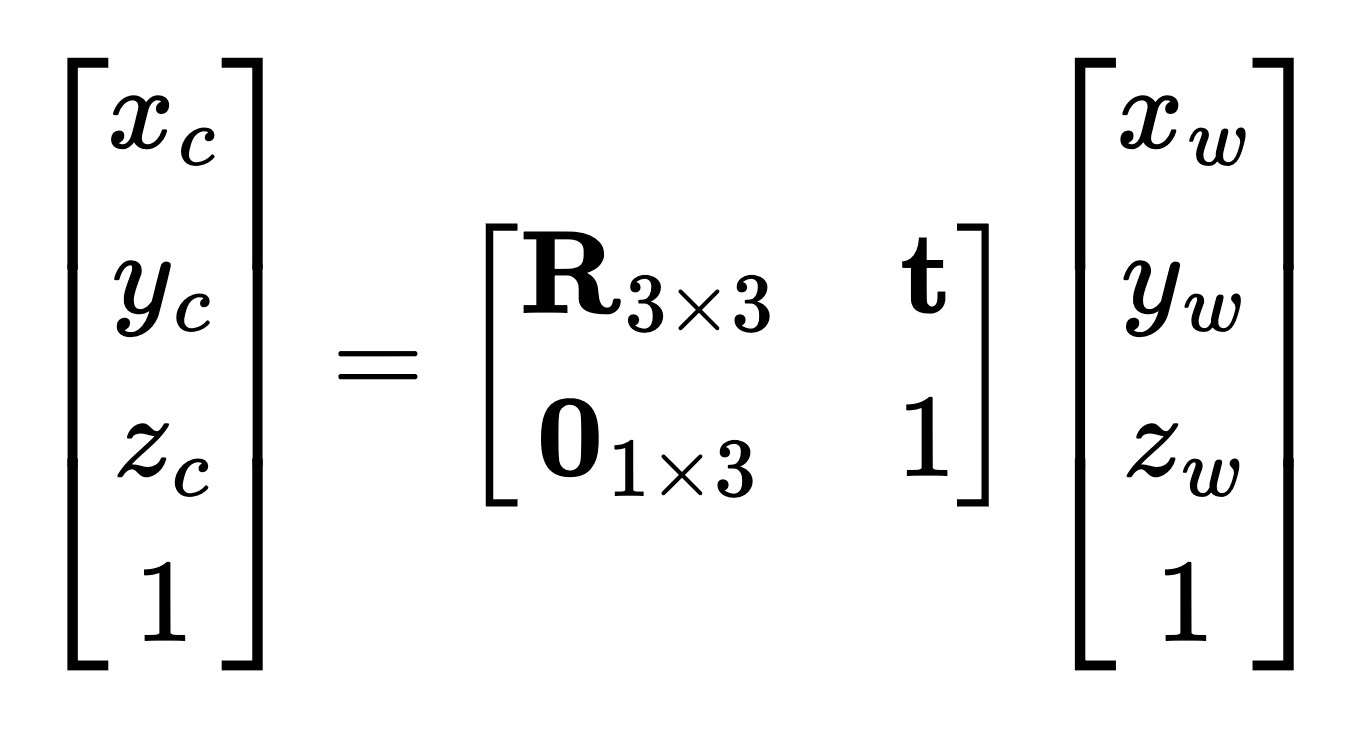
Relationship between world coordinates and camera coordinates
We can use the inverse of the matrix above to get the "c2w" matrix, which is luckily already provided to us in the training data.
Pixel coordinates in an image are converted to camera coordinates using the camera's intrinsic matrix. This matrix accounts for the focal length and principal point offset of the camera.
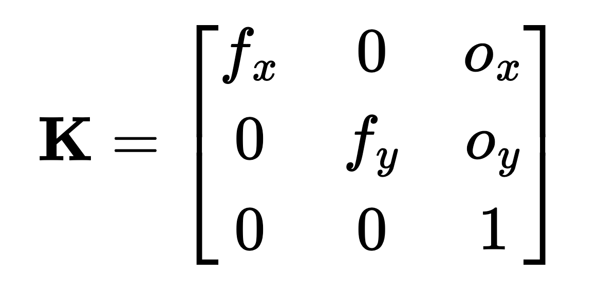
Camera Intrinsic Matrix, K
We can construct such a matrix and use it to convert image pixels in to camera coordinates
To convert pixel coordinates into rays:
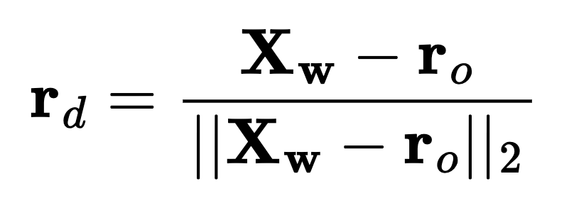
ray_o) is the camera's position in world coordinates, obtained directly from the extrinsic matrix.ray_d) is computed as the normalized vector pointing from the ray origin to the transformed world coordinate of the pixel.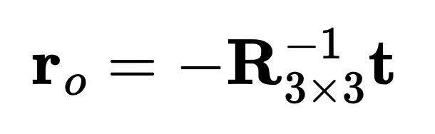
This results in a set of rays (ray_o, ray_d) for each pixel in the image. We then combine this with the color associated with each queried pixel to return the (ray_o, ray_d, color) tuples.
To efficiently train the NeRF model, we sample rays from images by selecting random pixels. This involves:
ray_o and ray_d) for the selected pixels.This approach ensures that the model is trained on diverse parts of the image while keeping memory usage manageable.
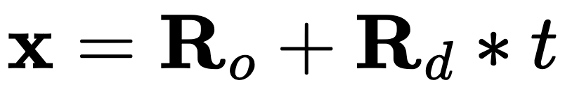
To feed the NeRF model, we sample 3D points along the rays by generating points spaced equally along it. This could be done by generating t values that are equally spaced from a specified depth range and calculating the following:
To prevent systematic overfitting, we can add some randomness to the T's generated to ensure we don't keep sampling the same points.
In this section, we integrate the components we've built so far to form a complete pipeline for sampling rays and visualizing them.
Now that we've implemented the ray sampling functionality, we can query a set of random rays from the input images. For each ray, we can sample a set of points along its path to be fed into the model. This process ensures that we have a diverse set of rays and corresponding 3D points that can be used for training the NeRF model.
Specifically, the ray sampler generates rays by selecting random pixels from the input image, converting these pixel coordinates into rays, and then sampling points along each ray. The resulting rays and sampled points are used as input for the model, helping it learn to generate realistic 3D reconstructions.
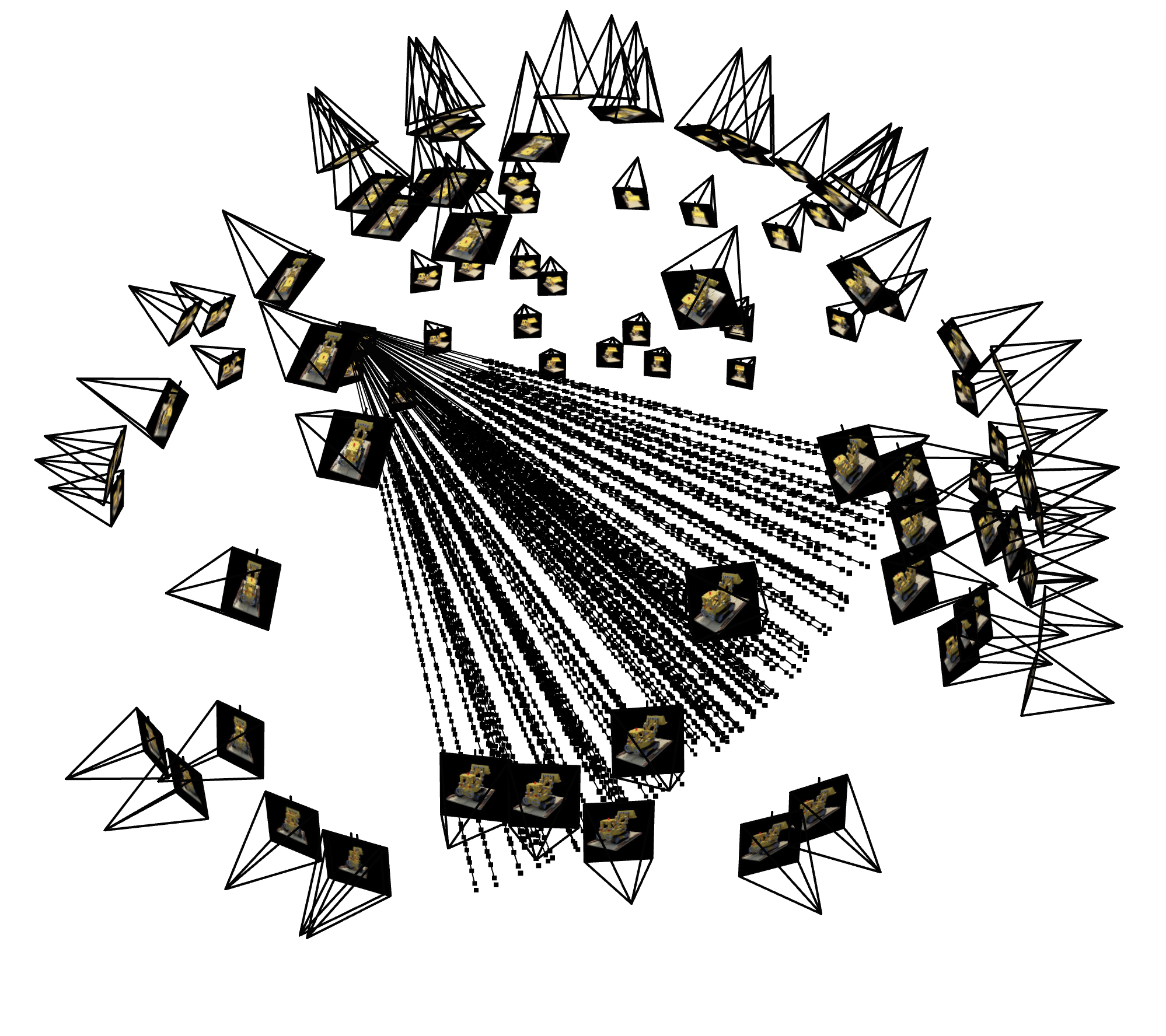
Once we have sampled the rays and points, we can visualize the results using Viser, an open-source software developed by NerfStudio. Viser provides a convenient way to visualize rays and sampled points in a 3D space. It renders the rays as lines and the sampled points as small spheres, making it easy to inspect the ray sampling process.
Viser also allows us to interactively explore the rays and sampled points, providing a deeper understanding of how the rays traverse the 3D scene. This visualization tool is essential for debugging and optimizing the sampling process.
We visualized the rays sampled randomly (from a random subsample of ~20 images) as well as the rays sampled from a single image for visualization purposes:
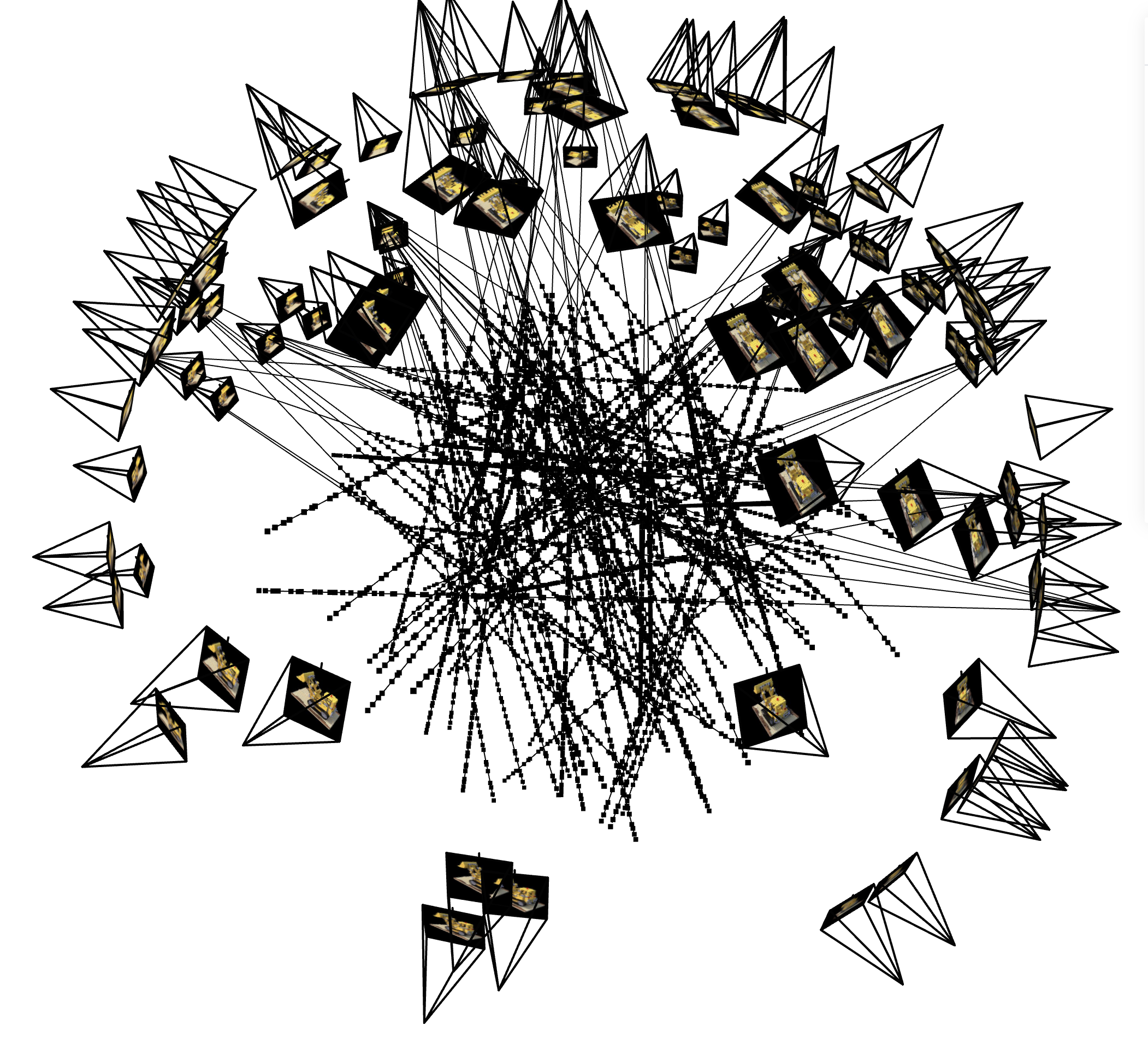
Rays Sampled From Plenty Images
Rays Sampled From One Image
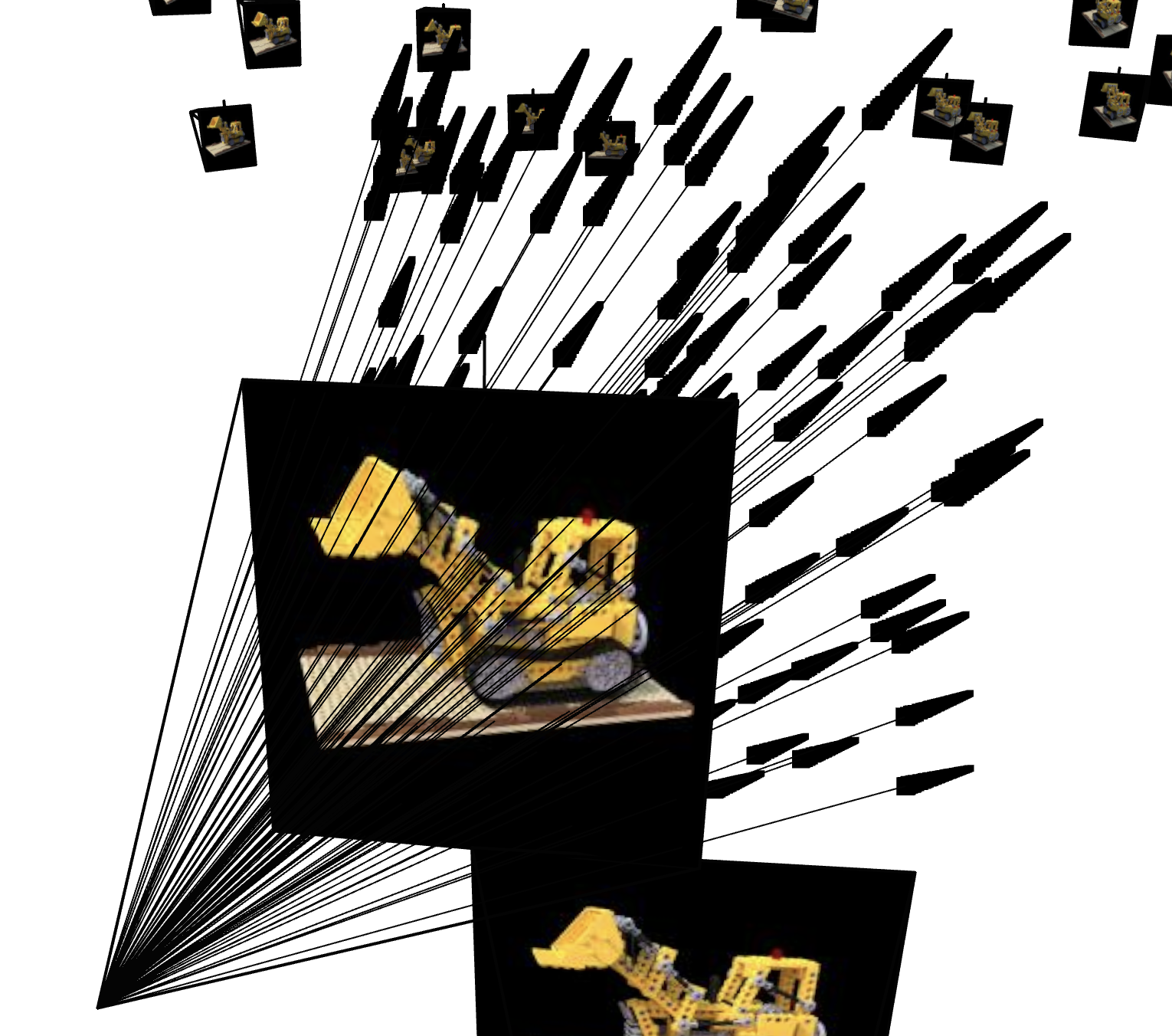
Close-Up of Single-Image Sampled Rays
In this section, we build a neural network model that extends the concepts from Part 1, but with key differences suited for 3D space. We list the differences as follows:
The specific model architecture details are shown as follows:
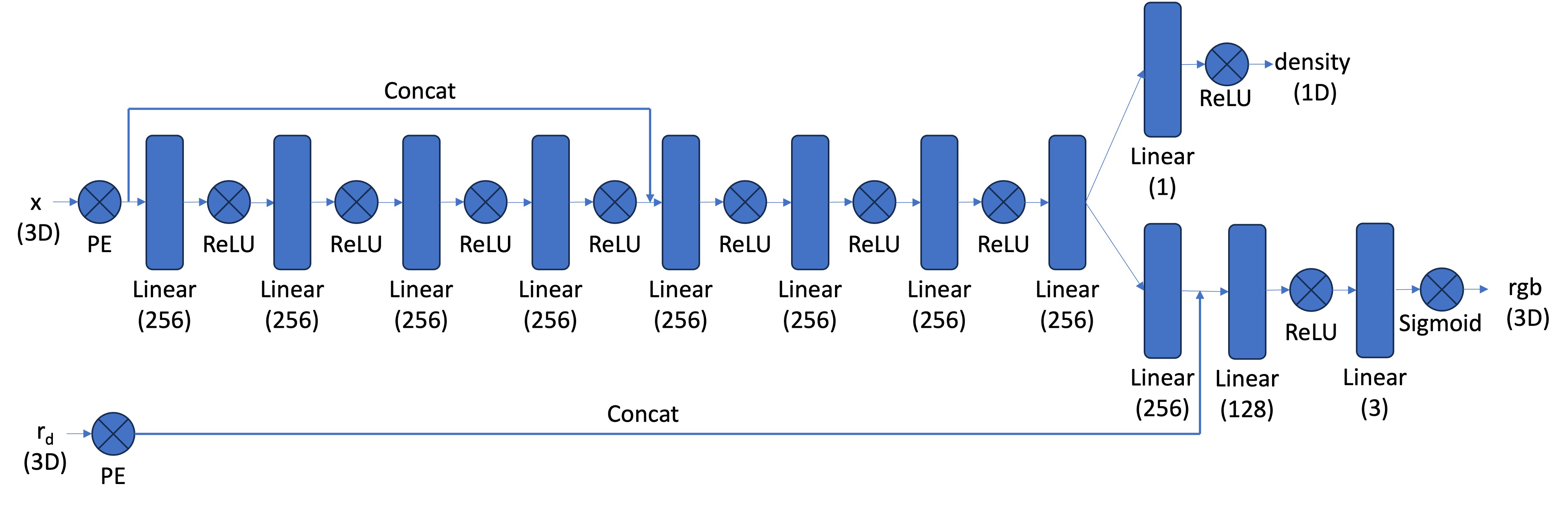
Model Architecture
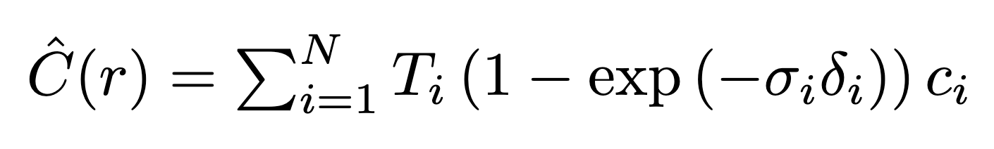
Volume rendering involves using the model's output to generate a realistic image by simulating how light travels through a scene. Given the model's output—RGB values and density at sampled points along each ray—we apply a rendering equation that takes into account the density and color along the ray to see what a view from that angle would look like. Explicitly we calculate it with the following:
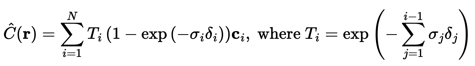
Discrete Volumetric Rendering Equation
Which is a discrete (and thus computable) version of the true volumetric rendering equation (which would otherwise feature an integral)
Using the function, we're able to render what the image would look like from a specified angle. We can use it to visualize how the model's generated image would look like throughout training.
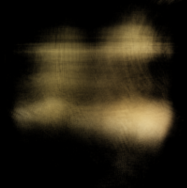
After 100 Steps
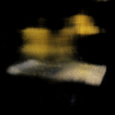
After 200 Steps
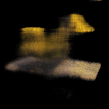
After 300 Steps
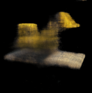
After 400 Steps
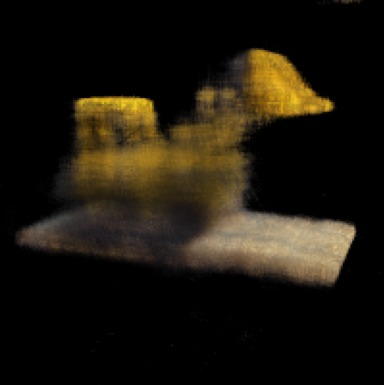
After 500 Steps

After 1000 Steps
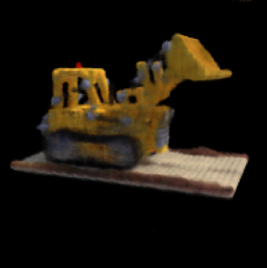
After 2500 Steps
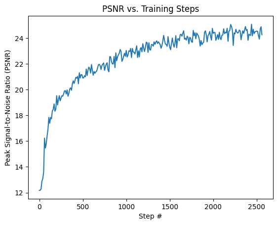
We can also track the PSNR values on the validation set throughout training and see it steadily increasing over time before reaching >24 PSNR near the end of training.
After fully training the network, we can also visualize the scene in a 360 manner using a novel test set of camera angles. We then generate a GIF by combining all the images together in a sequence.
Final Result
B&W Result
Lastly, for Bells and Whistles we can change the background color of the scene by modifying our volumetric rendering function as follows:
Original Volume Rendering Formula

Modified Volume Rendering Formula
Where cbg represents our desired background color.