
View of house in northside Berkeley (I)

View of house in northside Berkeley (II)
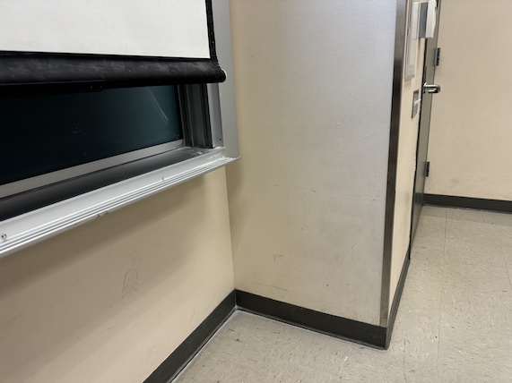
View of classroom while I was bored (I)
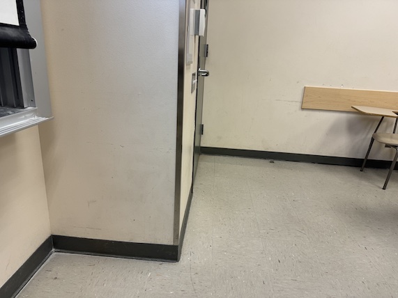
View of classroom while I was bored (II)
In this project I will be stiching together imagestaken from the same center of projection, similar to constructing a panorama from scratch.
I took a variety of images throughout the week leading up to this project. Here are the ones I ended up using:

View of house in northside Berkeley (I)

View of house in northside Berkeley (II)

View of classroom while I was bored (I)

View of classroom while I was bored (II)
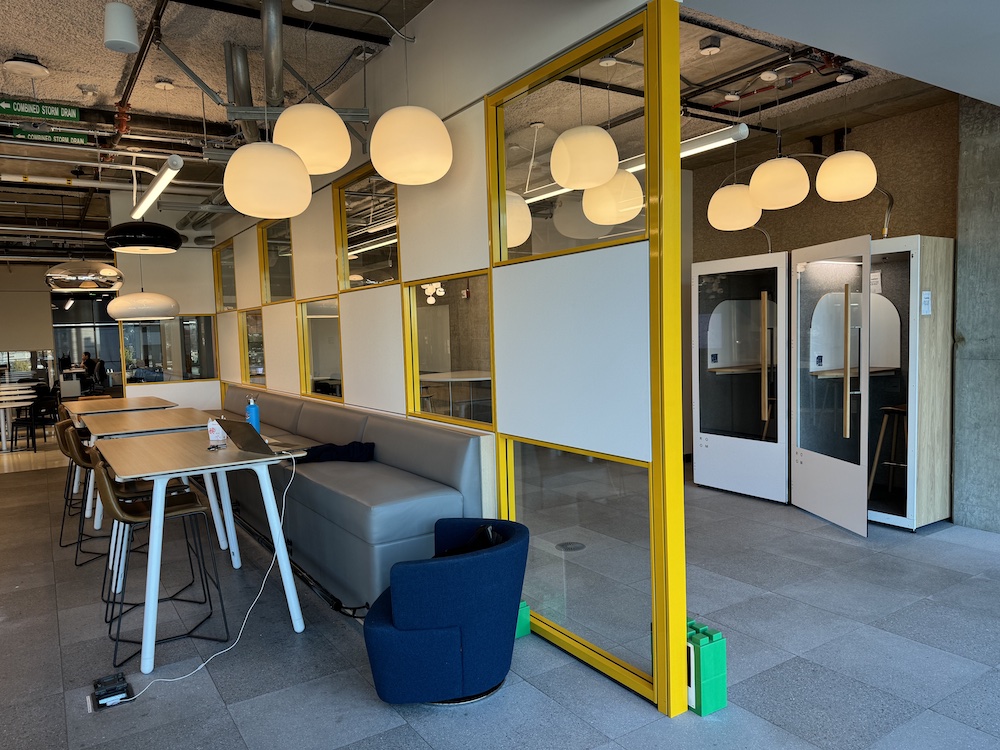
View of Berkeley Way West 8th Floor (I)
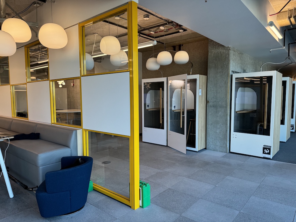
View of Berkeley Way West 8th Floor (II)
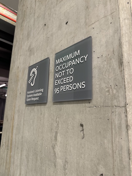
Picture of random sign
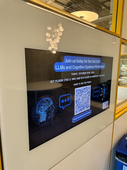
Picture of random LCD display
Similar to the previous project, we get correspondences between the images to be able to warp them to one another.
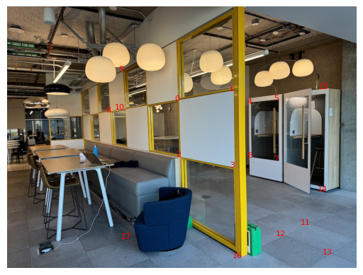
Point correspondences for first shot
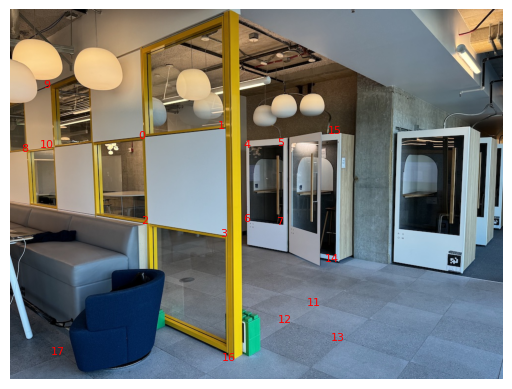
Point correspondences for second shot
The problem is, we no longer can do a triangular warp to align the images, but need something more powerful: a homography. A homography is another type of imaging warping method but this has 8 degrees of freedom instead of one. The entire warp matrix can be configured except for the bottom right corner, which must be 1. We can derrive a more straightforward matrix of coefficients to solve using least squares:
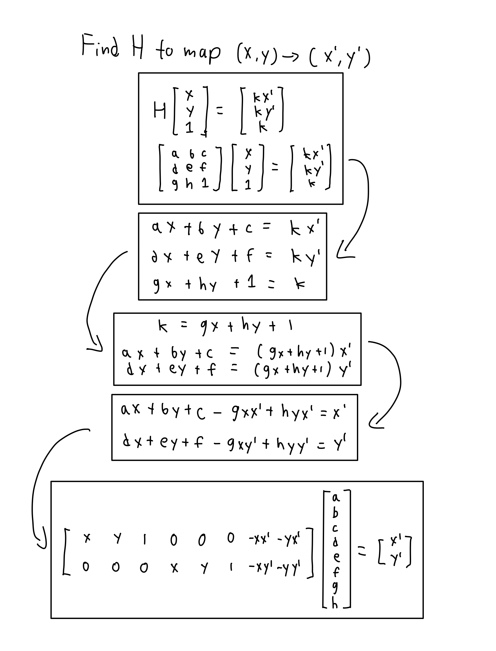
Once we solve for our homography matrix, we can warp the image as we please.

Right shot of lab
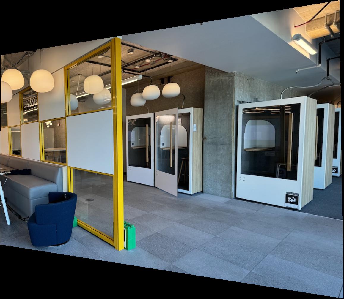
Right shot of lab warped to align with left shot
A neat thing we can do with our homographies is to rectify images. e.g. map square or rectangular surfaces into a flat projection. This can be done by calculating the homography using the surface's corners as the x, y and the flat coordinates as the x', y' like [(0, 0), (0, 100), (100, 0), (100, 100)].
Here are some examples of successful homographies.

Image of TV screen from an angle
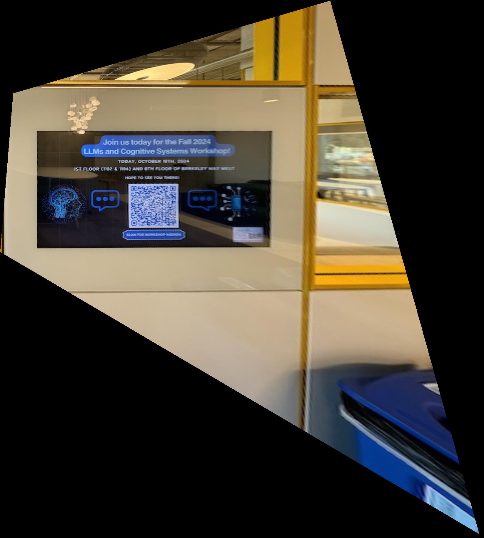
Rectified TV screen
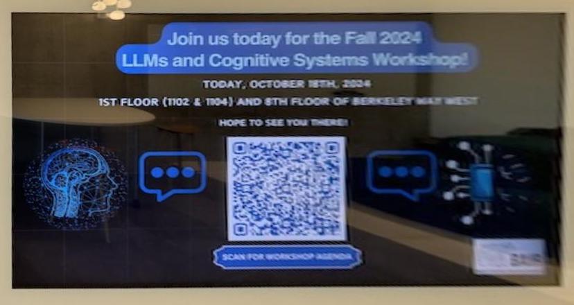
Cropped rectified TV screen

Image of sign from an angle
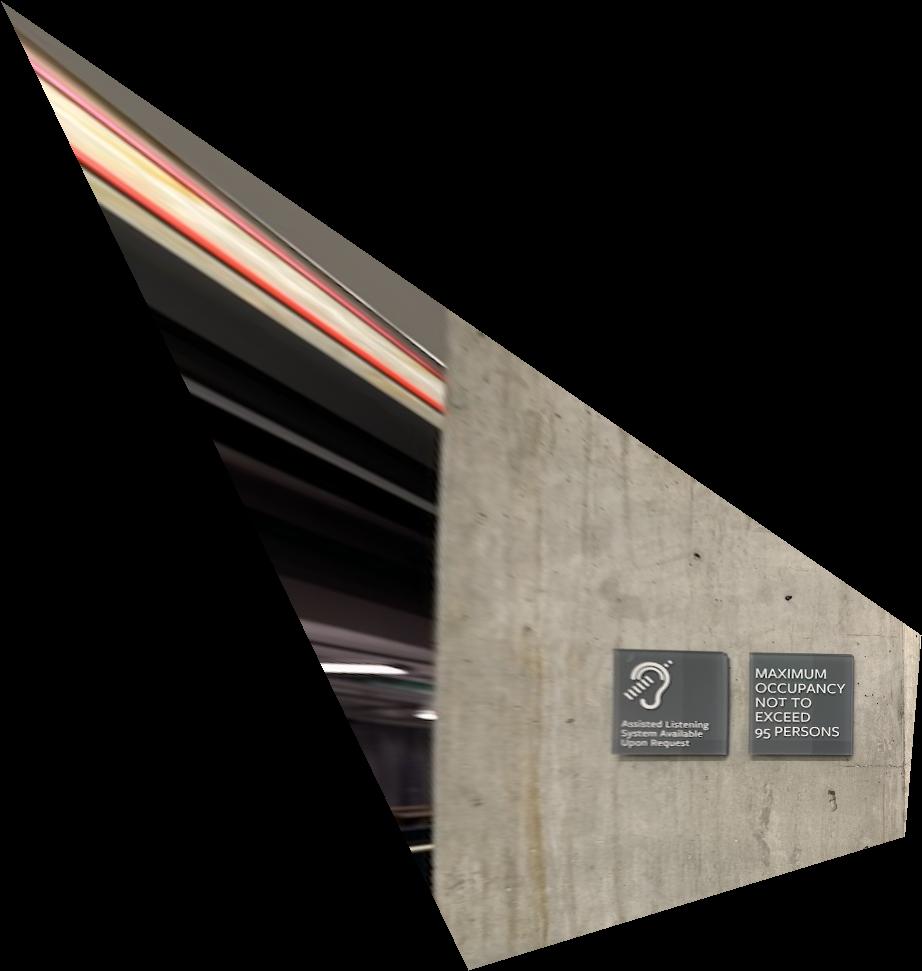
Rectified signage
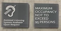
Cropped rectified signage
Using the homography and some clever alignment math, we can stich together images so they look like they're taken from the same perspective. I added an alpha chanel for the images to show where there is actually an image and when is it just empty space to pad the image. I used the alpha chanels to blend the images together when they both head content.

View of house in northside Berkeley (I)

View of house in northside Berkeley (II)
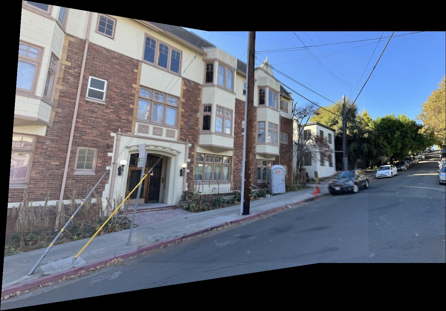
Blended view of house

View of classroom while I was bored (I)

View of classroom while I was bored (II)
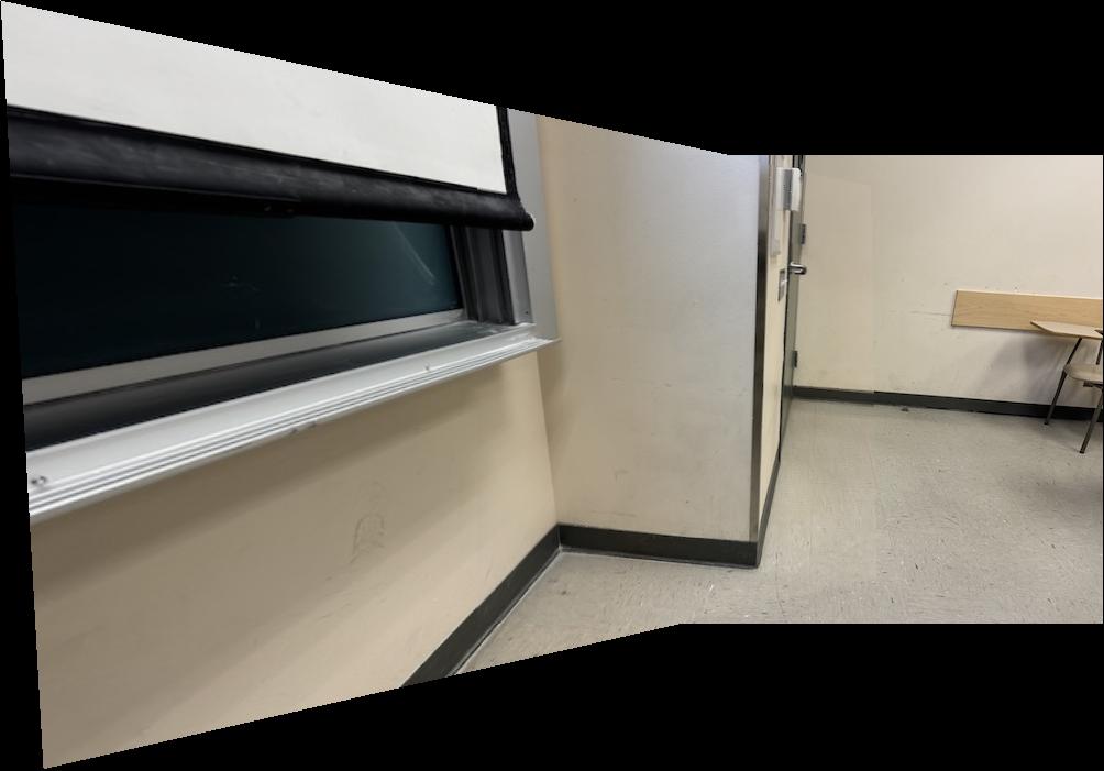
Blended view of classroom

View of Berkeley Way West 8th Floor (I)

View of Berkeley Way West 8th Floor (II)
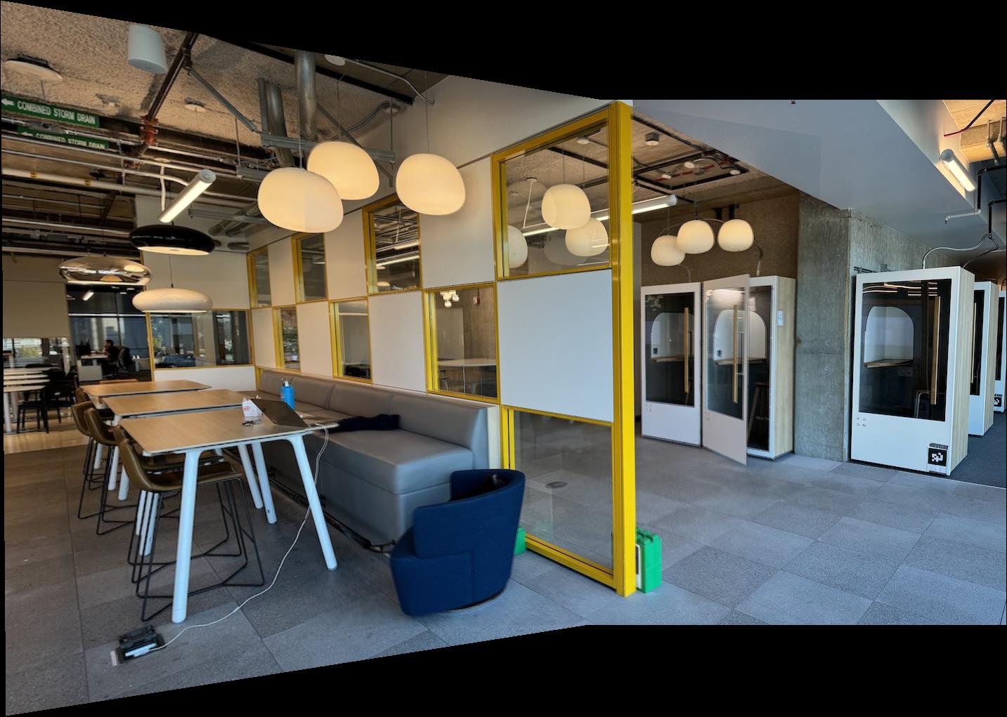
Blended view of BWW 8th Floor
Manual stitching works fine, but we can streamline the process significantly by automating the correspondence annotation. We can use some novel techniques to automatically detect features and calculate which ones match between images.
We can start by detecting corners using the Harris corner detector. We're interested in corners specifically because it's easier to see correspondences between images as they would look quite different when shifted in any direction. By using this corner detector, we can find many candidates for corners in the image. Let's try to do this on an imageo of an intersection near my house.
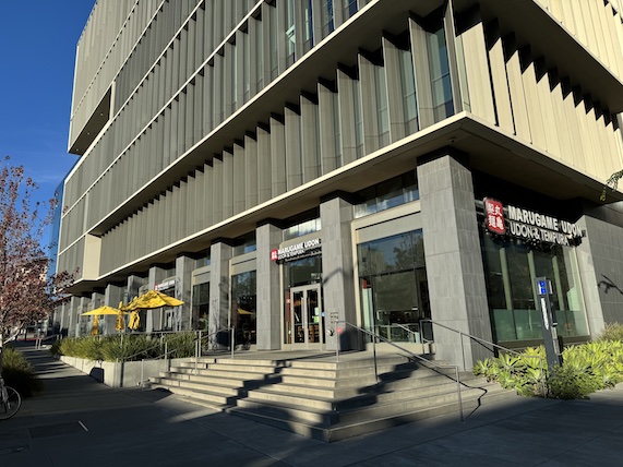
Left View
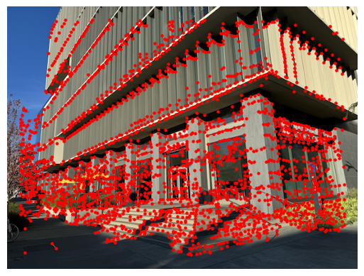
Left View with Harris Corners
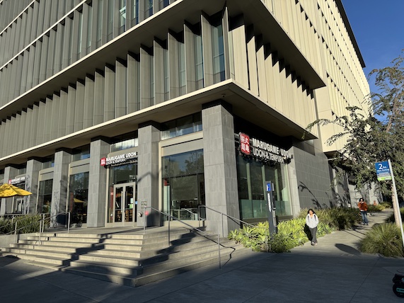
Right View
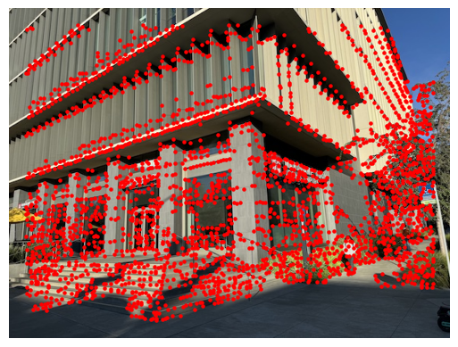
Right View with Harris Corners
This is great for giving us a good amount of corner candidates, however it is much too dense to plug into our next steps in the model because we'll have to the magnitude of 3-4 thousand points. We typically only need 500 or so for the next step of the process so need a way to downsample these points.
One straightforward method is to randomly sample but that could leave us with corner points with low "corner strength" values which was calculated from the Harris detector. We could also choose the top 500 points with the highest corner strength, however that could lead to many points being focused on certain areas of the image which isn't desirable because we would want a good distribution of the throughout. A solution to this is to use Adaptive Non-Maximal Suppression which takes both distance and corner strength into account when trying to select an optimal subset of points. This is the result of running ANMS on our 3k+ original corner candidates.

Left View with Harris Corners
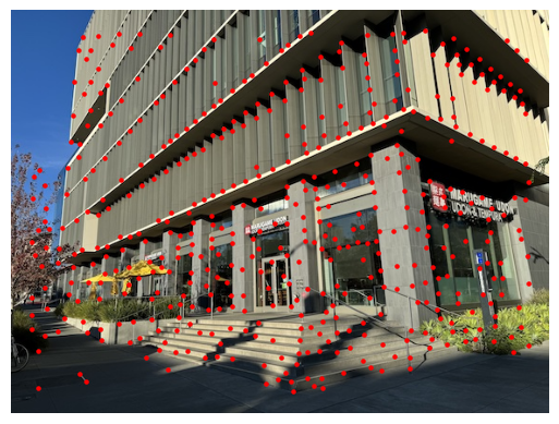
Harris Corners Narrowed Down with ANMS

Right View with Harris Corners
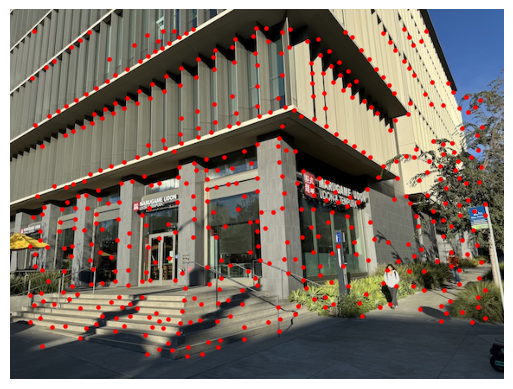
Harris Corners Narrowed Down with ANMS
Once we got a suitable set of corners, we now can start matching the points together between images to see which corners in image 1 correspond to which corners in image 2. The way we do this is by selecting a 40x40 window around each point, apply gaussian blur to make it a smaller 8x8 window, and essentially find the two corners in the other image with an 8x8 window that looks the most similar. Then we discard the ones that arent significantly more similar to its closest neighbor compared to their second closest neighbor. Doing this ensures points that don't have a good match are eliminated as they probably are outside of the overlapping range.
Here is what it looks like when we apply this procedure to match up the points:

Left Image Points

Right Image Points

Left Correspondences

Right Correspondences
However, there may still be some pesky little outliers remaining in our image. These would significantly affect the calculated homography because we calculate it using a least squares algorithm. Thus, we can eliminate these outliers through the following process: randomly subsample 4 points, use them to calculate a homography explicitly, then apply the homography to the remaining points and see if they are far off from the points they're supposed to be paired with, if they aren't label them as "inliers". Repeat this process a lot of times and find the homography with the largest number of inliers. This maximal set of inliers will be the final correspondences we can use to stitch together our homographies.

Initial Left Correspondences

Initial Right Correspondences
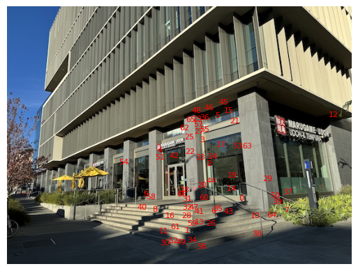
Left with Outliers Removed via RANSAC
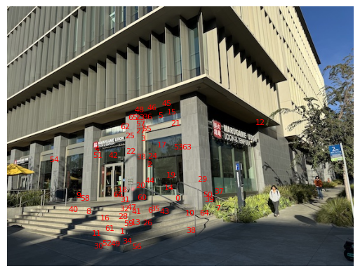
Right with Outliers Removed via RANSAC
The rest of the procedure is identical to the manual case and we can generate some nice complex mosaics now without needing to manually add the points.

Left View of Intersection

Right View of Intersection
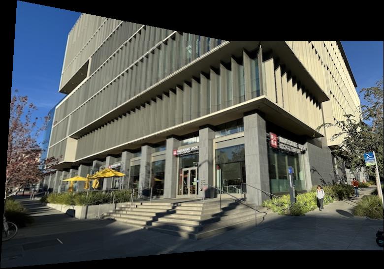
Intersection Stitched Together
Here are some other images I stitched together automatically!
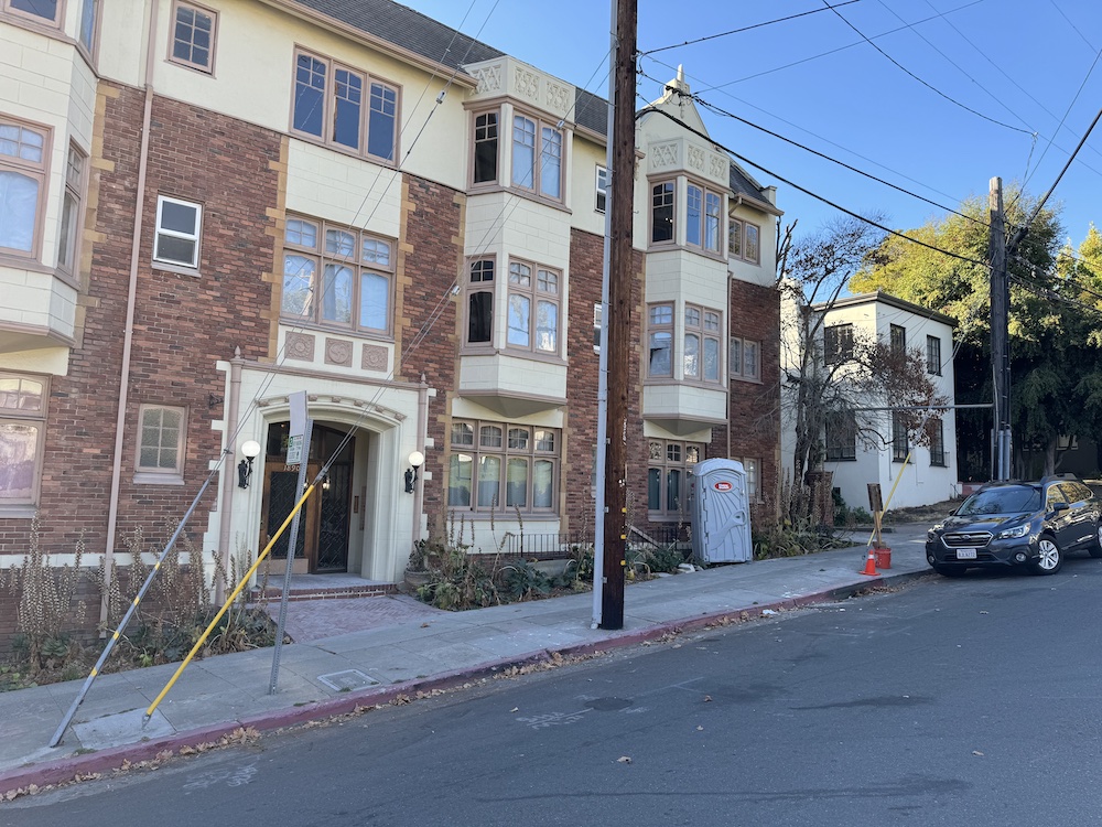
Houses Left View
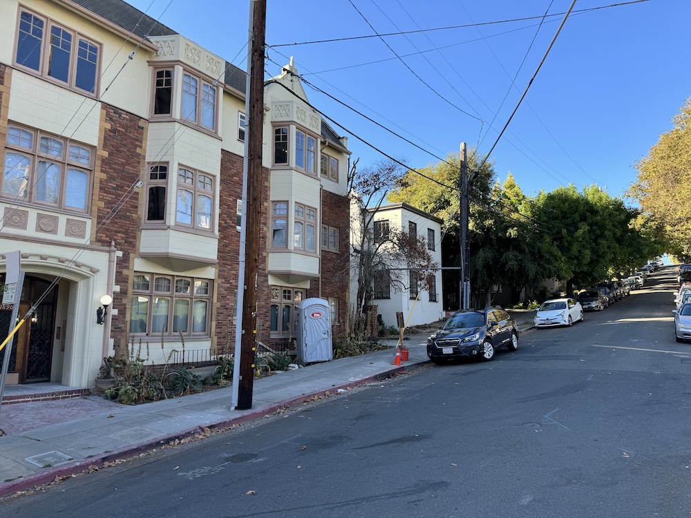
Houses Middle View
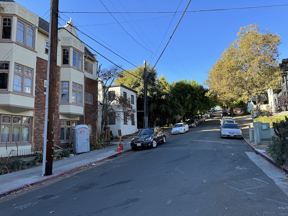
Houses Right View
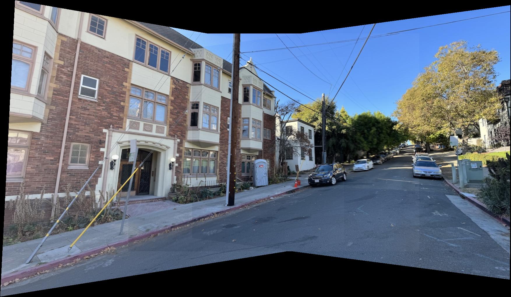
Houses Stitched
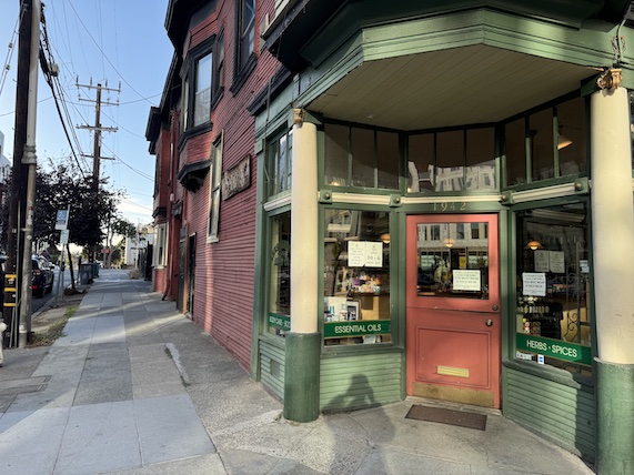
Herb Store Left View
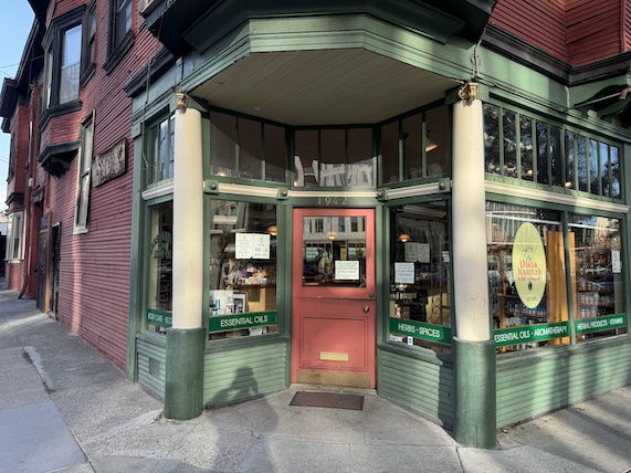
Herb Store Middle View
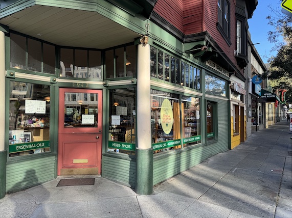
Herb Store Right View
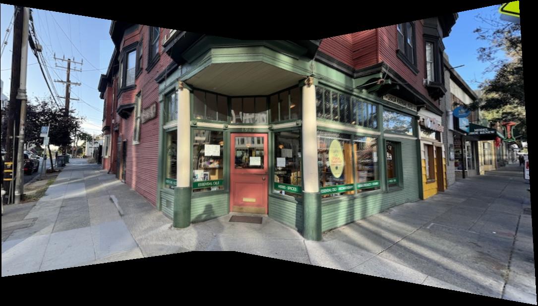
Herb Store Stitched
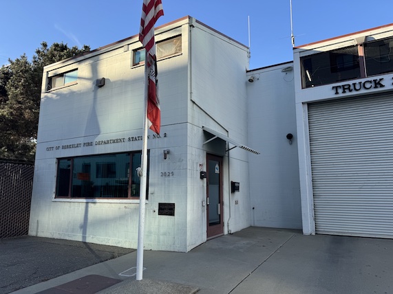
Fire Station View 1
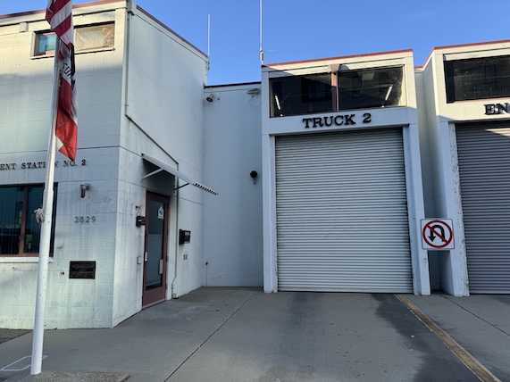
Fire Station View 2
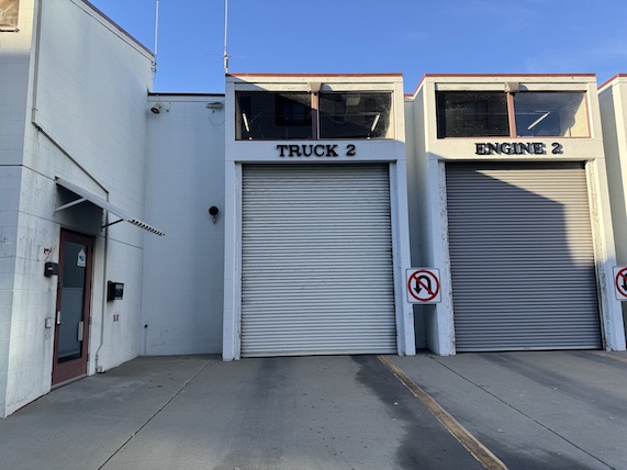
Fire Station View 3
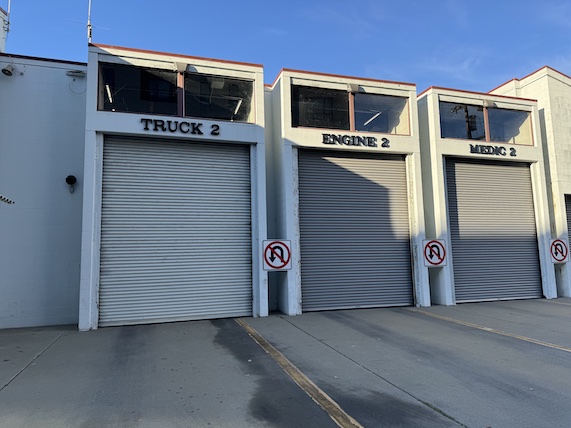
Fire Station View 4
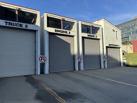
Fire Station View 5
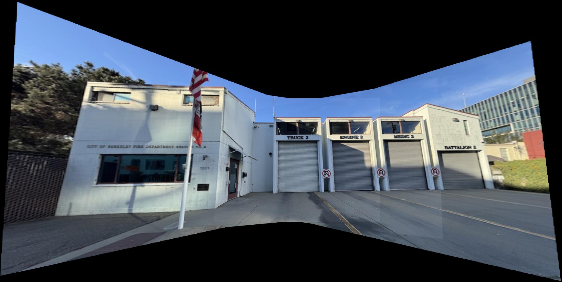
Fire Station Stitched
I think the biggest thing I learnt from this project is that I don't need to be worried about always implementing the most efficient solution from scratch. Sometimes it's better to get a basic version working and then iterating on it afterwards. I learnt this when doing the feature matching because I was stuck on designing a way to do the nearest neighbor searching efficiently without needing to gaussian blur it every time. Eventually I just implemented it and added caching with a dictionary and it worked just fine.